Easy IPCC part 1: Multi-Model Datatree
Handling heterogenous climate model data with xarray-datatree
Easy IPCC Part 1: Multi-Model Datatree
By Tom Nicholas (@TomNicholas) and Julius Busecke (@jbusecke)
(Originally posted on the Pangeo Medium blog)
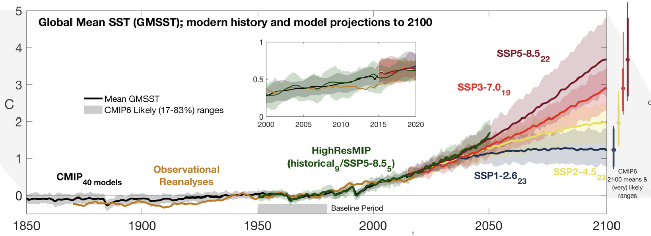
In this series of blog posts we aim to quickly reproduce a panel from one of the key figures (fig. 9.3a) of the IPCC AR6 Report from the raw climate model simulation data, using Pangeo cloud-native tools. This figure is critical: it literally shows our best estimate of the future state of the climate given certain choices by humanity.

This figure shows both the historical and projected global average temperature of the ocean’s surface, as used in different Global Climate Models. The projections are for possible trajectories of greenhouse gas emissions based on various socio-economic pathways (Neill et al. 2017).
However, the process of creating it is potentially very cumbersome: it involves downloading large files, idiosyncratic code to produce intermediate datafiles, and lots more code to finally plot the results. The open sharing of code used for the latest IPCC report inspired us to try to make this process easier for everyone.
The numerical model output produced under the Coupled Model Intercomparison Project 6 (CMIP6) output is publicly available (distributed by the Earth System Grid Federation), so the scientific community should be able to reproduce this plot from scratch, and then build upon it as the underlying science advances.
Due to recent advances in software and the migration of the CMIP6 data archive into the cloud, we are now able to produce this panel rapidly from raw data using easily available public cloud computing.
Working with many CMIP6 datasets at once can be cumbersome because each model has different size and coordinates. In this blogpost we highlight the new xarray-datatree package, which helps organize the many datasets in CMIP6 into a single tree-like data structure.
There have been other attempts to analyze, organize, and visualize multi-model experiments, but here we prioritize modularity, flexibility, extensibility, and using domain-agnostic tools.
We were able to reproduce parts of this graph in a live demo at Scipy 2022 using cloud-hosted data, but felt we could do it much more succinctly with datatree!
Getting the data
A key component of this workflow is having the large CMIP6 datasets available to open near-instantly from a public cloud store. The Pangeo/ESGF Cloud Data Working Group maintains Analysis-Ready Cloud-Optimized versions of a large part of the CMIP6 archive as Zarr stores as public datasets both on Google Cloud Storage and Amazon S3. (This alone is a huge advancement for open science, but just a part of what we’re showing today.)
For the sake of demonstration we will load a small subset of sea surface temperature data for three models . We’ll load both the historical baseline, as well as the SSP1.26 (“best case”) and SSP5.85 (“worst case”) future socio-economic pathways: a total of 9 datasets. (We’ll tackle scaling up to all the available data in a future blog post.)
import xarray as xr
xr.set_options(keep_attrs=True)
import gcsfs
from xmip.preprocessing import rename_cmip6

cmip_stores = {
'IPSL-CM6A-LR/historical':  'gs://cmip6/CMIP6/CMIP/IPSL/IPSL-CM6A-LR/historical/r4i1p1f1/Omon/tos/gn/v20180803/',
'MPI-ESM1-2-LR/historical': 'gs://cmip6/CMIP6/CMIP/MPI-M/MPI-ESM1-2-LR/historical/r4i1p1f1/Omon/tos/gn/v20190710/',
'CESM2/historical':         'gs://cmip6/CMIP6/CMIP/NCAR/CESM2/historical/r4i1p1f1/Omon/tos/gn/v20190308/',
'IPSL-CM6A-LR/ssp126':      'gs://cmip6/CMIP6/ScenarioMIP/IPSL/IPSL-CM6A-LR/ssp126/r4i1p1f1/Omon/tos/gn/v20191121/',
'IPSL-CM6A-LR/ssp585':      'gs://cmip6/CMIP6/ScenarioMIP/IPSL/IPSL-CM6A-LR/ssp585/r4i1p1f1/Omon/tos/gn/v20191122/',
'MPI-ESM1-2-LR/ssp126':     'gs://cmip6/CMIP6/ScenarioMIP/MPI-M/MPI-ESM1-2-LR/ssp126/r4i1p1f1/Omon/tos/gn/v20190710/',
'MPI-ESM1-2-LR/ssp585':     'gs://cmip6/CMIP6/ScenarioMIP/MPI-M/MPI-ESM1-2-LR/ssp585/r4i1p1f1/Omon/tos/gn/v20190710/',
'CESM2/ssp126':             'gs://cmip6/CMIP6/ScenarioMIP/NCAR/CESM2/ssp126/r4i1p1f1/Omon/tos/gn/v20200528/',
'CESM2/ssp585':             'gs://cmip6/CMIP6/ScenarioMIP/NCAR/CESM2/ssp585/r4i1p1f1/Omon/tos/gn/v20200528/'
}

datasets = {
    name: rename_cmip6(xr.open_dataset(path, engine="zarr")).load()
    for name, path in cmip_stores.items()
}
CMIP vocabulary explainer: The words “model” and “experiment” have a specific meaning in CMIP lingo. Within CMIP there are many different datasets produced by various modeling centers around the world. Each of these centers has one or more model setups (
source_idin official CMIP language), which are used to produce multiple simulations. For example the simulations forIPSL-CM6A-LRare all produced by the Institut Pierre-Simon Laplace in France. Different simulations are run under certain protocols which prescribe conditions (e.g. greenhouse gas forcings), and these are called experiments. The experiments we’ve loaded here are'historical','ssp126'&'ssp585'.
These nine datasets are all similar, e.g. they have the same dimension names (freshly cleaned thanks to another package of ours - xMIP) and variable names, but they have different sizes along dimensions: horizontal dimensions differ due to varying resolution and time dimensions differ because the historical baseline run is longer than the scenarios by a varying amount.
print(datasets["CESM2/ssp585"].sizes)
print(datasets["IPSL-CM6A-LR/ssp585"].sizes)
Frozen({'y': 384, 'x': 320, 'vertex': 4, 'time': 1032, 'bnds': 2})
Frozen({'y': 332, 'x': 362, 'vertex': 4, 'time': 1032, 'bnds': 2})
For instance the "x" and "y" dimensions here (roughly corresponding to latitude and longitude) do not match between the CESM2 model and the IPSL model. Hence they cannot be combined into a single N-dimensional array or a single xarray.Dataset!
Introducing datatree
The CMIP6 datasets are clearly related, however. They have a hierarchical order - grouped by model and then by experiment. Each dataset also contains very similar variables. Wouldn’t it be nice to treat them all as one related set of data, and analyze them together?
The xarray-datatree package enables this. It arranges these related datasets into a Datatree object, allowing them to be manipulated together. A DataTree object can be thought of as a recursive dictionary of xarray.Dataset objects, with additional methods for performing computations on the entire tree at once. You can also think of it as an in-memory representation of an entire netCDF file, including all netCDF groups. Because it is in-memory your analysis does not require saving intermediate files to disk.
Note: The pip-installable package
xarray-datatreeprovides the classDataTree, importable from the moduledatatree. From here on we will refer interchangeably to these as just “datatree”.
from datatree import DataTree

dt = DataTree.from_dict(datasets)

print(f"Size of data in tree = {dt.nbytes / 1e9 :.2f} GB")
Size of data in tree = 4.89 GB
print(dt)
DataTree('None', parent=None)
├── DataTree('IPSL-CM6A-LR')
│   ├── DataTree('historical')
│   │       Dimensions:      (y: 332, x: 362, vertex: 4, time: 1980, bnds: 2)
│   │       Coordinates:
│   │         * time         (time) object 1850-01-16 12:00:00 ... 2014-12-16 12:00:00
│   │       Dimensions without coordinates: y, x, vertex, bnds
│   │       Data variables:
│   │           area         (y, x) float32 16.0 16.0 16.0 ... 1.55e+08 3.18e+07 3.18e+07
│   │           lat_bounds   (y, x, vertex) float32 -84.21 -84.21 -84.21 ... 50.11 49.98
│   │           lon_bounds   (y, x, vertex) float32 72.5 72.5 72.5 72.5 ... 73.0 72.95 73.0
│   │           lat          (y, x) float32 -84.21 -84.21 -84.21 ... 50.23 50.01 50.01
│   │           lon          (y, x) float32 72.5 73.5 74.5 75.5 ... 73.05 73.04 73.0 72.99
│   │           time_bounds  (time, bnds) object 1850-01-01 00:00:00 ... 2015-01-01 00:00:00
│   │           tos          (time, y, x) float32 nan nan nan nan nan ... nan nan nan nan
│   │       Attributes: (12/54)
│   │           CMIP6_CV_version:       cv=6.2.3.5-2-g63b123e
│   │           Conventions:            CF-1.7 CMIP-6.2
│   │           EXPID:                  historical
│   │           NCO:                    "4.6.0"
│   │           activity_id:            CMIP
│   │           branch_method:          standard
│   │           ...                     ...
│   │           tracking_id:            hdl:21.14100/dc824b97-b288-4ec0-adde-8dbcfa3b0095
│   │           variable_id:            tos
│   │           variant_label:          r4i1p1f1
│   │           status:                 2019-11-09;created;by nhn2@columbia.edu
│   │           netcdf_tracking_ids:    hdl:21.14100/dc824b97-b288-4ec0-adde-8dbcfa3b0095
│   │           version_id:             v20180803
│   ├── DataTree('ssp126')
│   │       Dimensions:      (y: 332, x: 362, vertex: 4, time: 1032, bnds: 2)
│   │       Coordinates:
│   │         * time         (time) object 2015-01-16 12:00:00 ... 2100-12-16 12:00:00
│   │       Dimensions without coordinates: y, x, vertex, bnds
│   │       Data variables:
│   │           area         (y, x) float32 16.0 16.0 16.0 ... 1.55e+08 3.18e+07 3.18e+07
│   │           lat_bounds   (y, x, vertex) float32 -84.21 -84.21 -84.21 ... 50.11 49.98
│   │           lon_bounds   (y, x, vertex) float32 72.5 72.5 72.5 72.5 ... 73.0 72.95 73.0
│   │           lat          (y, x) float32 -84.21 -84.21 -84.21 ... 50.23 50.01 50.01
│   │           lon          (y, x) float32 72.5 73.5 74.5 75.5 ... 73.05 73.04 73.0 72.99
│   │           time_bounds  (time, bnds) object 2015-01-01 00:00:00 ... 2101-01-01 00:00:00
│   │           tos          (time, y, x) float32 nan nan nan nan nan ... nan nan nan nan
...
We created the whole tree in one go from our dictionary of nine datasets, using the keys of the dict to organize the resulting tree. DataTree objects are structured similarly to a UNIX filesystem, so a key in the dict such as 'IPSL-CM6A-LR/historical' will create a node called IPSL-CM6A-LR and another child node below it called 'historical'. This approach means the DataTree.from_dict method can create trees of arbitrary complexity from flat dictionaries.
If instead we wanted to create the tree manually, you can do that by setting the
.childrenattributes of each node explicitly, assigning other tree objects to build up a composite result.
You can see that the resulting tree structure is grouped by model first, and then by the experiment. (This choice is somewhat arbitrary and we could have chosen to group first by experiment and then model.)
While we printed the string representation of the tree for this blog post, if you’re doing this in a jupyter notebook you will actually automatically get an interactive HTML representation of the tree, where each node is collapsible.
We say that we have created one “tree”, where each “node” within that tree (optionally) contains the contents of exactly one xarray.Dataset, and also has a node name, a “parent” node, and can have any number of “child” nodes. For more information on the data model datatree uses, see the documentation.
We can actually access nodes in the tree using path-like syntax too, for example
print(dt["/CESM2/ssp585"])
DataTree('ssp585', parent="CESM2")
    Dimensions:      (y: 384, x: 320, vertex: 4, time: 1032, bnds: 2)
    Coordinates:
      * y            (y) int32 1 2 3 4 5 6 7 8 9 ... 377 378 379 380 381 382 383 384
      * x            (x) int32 1 2 3 4 5 6 7 8 9 ... 313 314 315 316 317 318 319 320
      * time         (time) object 2015-01-15 13:00:00 ... 2100-12-15 12:00:00
    Dimensions without coordinates: vertex, bnds
    Data variables:
        lat          (y, x) float64 -79.22 -79.22 -79.22 -79.22 ... 72.2 72.19 72.19
        lat_bounds   (y, x, vertex) float32 -79.49 -79.49 -78.95 ... 72.41 72.41
        lon          (y, x) float64 320.6 321.7 322.8 323.9 ... 318.9 319.4 319.8
        lon_bounds   (y, x, vertex) float32 320.0 321.1 321.1 ... 320.0 320.0 319.6
        time_bounds  (time, bnds) object 2015-01-01 02:00:00.000003 ... 2101-01-0...
        tos          (time, y, x) float32 nan nan nan nan nan ... nan nan nan nan
    Attributes: (12/48)
        Conventions:            CF-1.7 CMIP-6.2
        activity_id:            ScenarioMIP
        branch_method:          standard
        branch_time_in_child:   735110.0
        branch_time_in_parent:  735110.0
        case_id:                1735
        ...                     ...
        tracking_id:            hdl:21.14100/68b741c9-b8f8-479d-b48c-6853b1c71e56...
        variable_id:            tos
        variant_info:           CMIP6 SSP5-8.5 experiments (2015-2100) with CAM6,...
        variant_label:          r4i1p1f1
        netcdf_tracking_ids:    hdl:21.14100/68b741c9-b8f8-479d-b48c-6853b1c71e56...
        version_id:             v20200528
You can see that every node is itself another DataTree object, i.e. the tree is a recursive data structure.
This structure not only allows the user full flexibility in how to set up and manipulate the tree, but it also behaves like a filesystem that people are already very familiar with.
But datatrees are not just a neat way to organize xarray datasets; they also allows us to operate on datasets in an intuitive way.
Timeseries
In this case the basic quantity we want to compute is a global mean of the ocean surface temperature. For this we can use the built-in .mean() method.
timeseries = dt.mean(dim=["x", "y"])
This works exactly like the familiar xarray method, and averages the temperature values over the horizontal dimensions for each dataset on any level of the tree. :exploding_head:
All arguments are passed down, so this .mean will work so long as the data in each node of the tree has a "x" and a "y" dimension to average over.
Lets confirm our results by plotting a single dataset from the new tree of timeseries:
timeseries['/IPSL-CM6A-LR/ssp585'].ds['tos'].plot()

And indeed, we get a nice timeseries. Once you select a node, you get back an xarray.Dataset using .ds and can do all the good stuff you already know (like plotting).
For comparison, here is the relevant part of Julius’ code from the Scipy 2022 live demo that did not use datatree:
timeseries_hist_datasets = []
timeseries_ssp126_datasets = []
timeseries_ssp245_datasets = []
timeseries_ssp370_datasets = []
timeseries_ssp585_datasets = []

for k,ds in data_timeseries.items():
    # Separate experiments
    out = ds.convert_calendar('standard')
    out = out.sel(time=slice('1850', '2100'))# cut extended runs
    out = out.assign_coords(source_id=ds.source_id)
    if ds.experiment_id == 'historical':
        # CMIP
        if len(out.time)==1980:
            timeseries_hist_datasets.append(out)
        else:
            print(f"found {len(ds.time)} for {k}")
    else:
        #scenarioMIP
        if len(out.time)!=1032:
            print(f"found {len(out.time)} for {k}")
            # print(ds.time)
        else:
            if ds.experiment_id == 'ssp126':
                timeseries_ssp126_datasets.append(out)
            elif ds.experiment_id == 'ssp245':
                timeseries_ssp245_datasets.append(out)
            elif ds.experiment_id == 'ssp370':
                timeseries_ssp370_datasets.append(out)
            elif ds.experiment_id == 'ssp585':
                timeseries_ssp585_datasets.append(out)

concat_kwargs = dict(
    dim='source_id',
    join='override',
    compat='override',
    coords='minimal'
)
timeseries_hist = xr.concat(timeseries_hist_datasets, **concat_kwargs)
timeseries_ssp126 = xr.concat(timeseries_ssp126_datasets, **concat_kwargs)
timeseries_ssp245 = xr.concat(timeseries_ssp245_datasets, **concat_kwargs)
timeseries_ssp370 = xr.concat(timeseries_ssp370_datasets, **concat_kwargs)
timeseries_ssp585 = xr.concat(timeseries_ssp585_datasets, **concat_kwargs)
😬 Definitely not as nice as a one-liner…
It’s worth understanding what happened under the hood when calling .mean() on the tree. We can reproduce the behavior of .mean() by passing a simple function to the built-in .map_over_subtree() method.
def mean_over_space(ds):
    return ds.mean(dim=["x", "y"])

dt.map_over_subtree(mean_over_space)
The function mean_over_space that we supplied gets applied to the data in each and every node in the tree automatically. This will return the exact same result as above, but with this method users can map arbitrary functions over each dataset in the tree, as long as they consume and produce xarray.Datasets. You can even map functions with multiple inputs and outputs, but that is an advanced use case which we will use at the end of this post.
You can already see that this enables very intuitive mapping of custom functions without lengthy writing of loops.
Saving output
Before we go further, we might want to save our aggregated timeseries data to use later. DataTree supports saving to and loading from both netCDF files and Zarr stores.
from datatree import open_datatree

timeseries.to_zarr('cmip_timeseries')  # or netcdf, with any group structure

roundtrip = open_datatree('cmip_timeseries', engine="zarr")
print(roundtrip)
DataTree('None', parent=None)
├── DataTree('CESM2')
│   ├── DataTree('historical')
│   │       Dimensions:      (vertex: 4, time: 1980, bnds: 2)
│   │       Coordinates:
│   │         * time         (time) object 1850-01-15 12:59:59.999997 ... 2014-12-15 12:0...
│   │       Dimensions without coordinates: vertex, bnds
│   │       Data variables:
│   │           lat          float64 ...
│   │           lat_bounds   (vertex) float32 ...
│   │           lon          float64 ...
│   │           lon_bounds   (vertex) float32 ...
│   │           time_bounds  (time, bnds) object ...
│   │           tos          (time) float32 ...
...
Nodes are saved as netCDF or Zarr groups, meaning that you can now work smoothly with xarray and multi-group files, a long-term sticking point for many xarray users. Being able to now work with such files without leaving xarray or python helps retains backwards compatibility and portability.
Calculating anomalies
Note on Climate Anomalies: Coupled climate models often exhibit ‘biases’, which means that the ocean temperatures at the starting point for e.g. the historical and future experiments will differ from model to model. For the purpose of this scientific analysis however we are most interested in the relative change from that starting point when a forcing (e.g. increased greenhouse gases) is applied. Conventionally we compute the anomaly relative to a given reference value. In this case the reference value is the global ocean temperature averaged over the years 1950-1980 in the corresponding historical experiment. Therefore we want to compute and subtract this reference value for each model separately so that each model-specific bias is removed.
In practice we need to iterate over each model, pick the historical experiment, select the base period, and average it. We then subtract that resulting value from all experiments of the corresponding model and rearrange the resulting anomaly timeseries into a new tree.
anomaly = DataTree()
for model_name, model in timeseries.children.items():

    # model-specific base period as an xarray.Dataset
    base_period = model["historical"].ds.sel(time=slice('1950','1980')).mean('time')

    anomaly[model_name] = model - base_period   # subtree - Dataset
We have used a few features of datatree here. We loop over the .children attribute of the DataTree, which iterates through each sub-node in turn in a dictionary-like manner.
We find the reference value (base_period) by extracting the data in a node as an xarray.Dataset via .ds, giving us access to all of xarray’s normal API for computations.
Our tree of results (anomaly) is constructed by creating an empty tree and then adding branches to this new tree whilst we loop through models.
In the final line of this for loop we have subtracted an xarray.Dataset from a DataTree - this operation works node-wise, i.e. the dataset is subtracted from every data-containing node in the tree.
Note: In general, we could imagine having rules for operations involving any number of trees of any node structure, analogous to numpy array broadcasting. This would make the above anomaly calculation much more succinct. However at the moment, datatree only supports
tree @ dataset-like operations andtree @ tree-like operations, where the trees must have the same node structure.
Plotting
Alright, so the final step here is to actually plot the data. We can use the map_over_subtree approach to plot each individual simulation onto the same matplotlib axes:
import matplotlib.pyplot as plt

from datatree import map_over_subtree

fig, ax = plt.subplots()


@map_over_subtree
def plot_temp(ds, original_ds):

    if ds:
        label = f'{original_ds.attrs["source_id"]} - {original_ds.attrs["experiment_id"]}'
        ds['tos'].rolling(time=2*12).mean().plot(ax=ax, label=label)

    return ds


plot_temp(anomaly, timeseries)
ax.legend()

For this we created a matplotlib figure and axis and then used the built-in xarray plotting capability to add each timeseries to the existing matplotlib.Axes object.
Instead of using the .map_over_subtree method on the DataTree class, we instead used map_over_subtree as a function decorator, which promoted plot_temp to a function that will act over all nodes of any given tree. This decorator is happy to map over multiple trees simultaneously, which we used to extract the metadata for labelling each timeseries.
Note: The way we extracted this metadata for plotting was a little awkward - we can imagine improving this in future versions of datatree.
The fact that we operate on an xarray dataset also allows us to convieniently smooth the timeseries (by a 2 year rolling mean) to remove the seasonal cycle.
Looking at the figure produced above, we’ve successfully replicated the basic features of the IPCC plot that we wanted! And it took us very few lines of code overall, especially compared to how it’s often done. In future posts we will improve this figure, adding more data and maybe making it interactive.
(Eagle-eyed climate scientist readers will have noticed that our figure is not actually quite correct - we forgot to correctly weight our temperature averages by the areas of the grid cells in each model! We will deal with this subtlety and other more complex custom aggregations in a future blog post.)
Takeaways
Datatree is a general tool. Whilst here we used it on CMIP6 data, we learnt about capabilities that might be useful in other projects. We saw that datatree can:
- Organize heterogeneous data
- Seamlessly extend xarray’s functionality
- Handle I/O with nested groups
- Apply operations over whole trees
- Perform more complex and custom operations
- Retain fine-grained control
- Reduce overall lines of code
Future
This blogpost is the first in a series. We plan to write more to discuss:
- Using intake with datatree, where the trees could act like in-memory catalogs,
- Suporting more complex aggregation operations, such as using
.weightedto weight an operation on one tree with weights from another tree, - Scaling out to a much larger set of CMIP6 data with dask,
- Quick plotting of data in a whole tree, maybe even making it interactive.